PBDL Dataloader Project

It is also worth highlightig our new PBDL dataloader project: https://github.com/tum-pbs/pbdl-dataset, created by TUM Bachelor student Sebastian Pfister. It provides convenient access to our datasets.

Our “classic” airfoil learning example using the loader can be found under the link below. It is very concise now: https://colab.research.google.com/github/tum-pbs/pbdl-book/blob/master/supervised-airfoils.ipynb

The current content is:

  • Incompressible Navier-Stokes wake flow over time
  • Transonic (compressible) cylinder flow
  • A simple NS wake flow (Solver-in-the-Loop)
  • Kuramoto-Sivashinsky in 1D (chaotic)
  • and a Reynolds-averaged airfoil flow data set.

More datasets to come in the next weeks! 😀


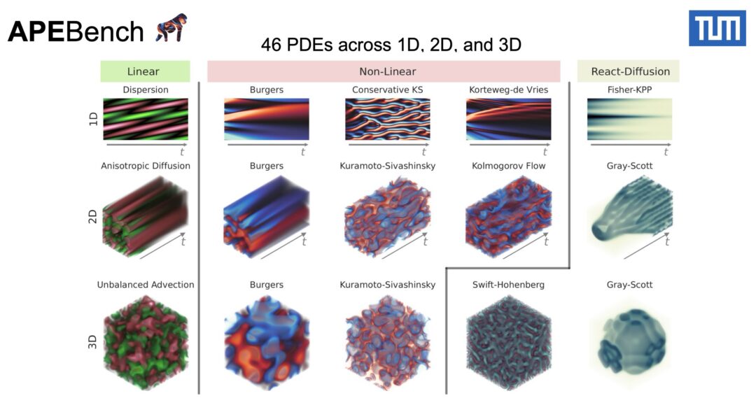
🦧 APEBench 🦍 A Benchmark for Autoregressive Neural Emulators of PDEs

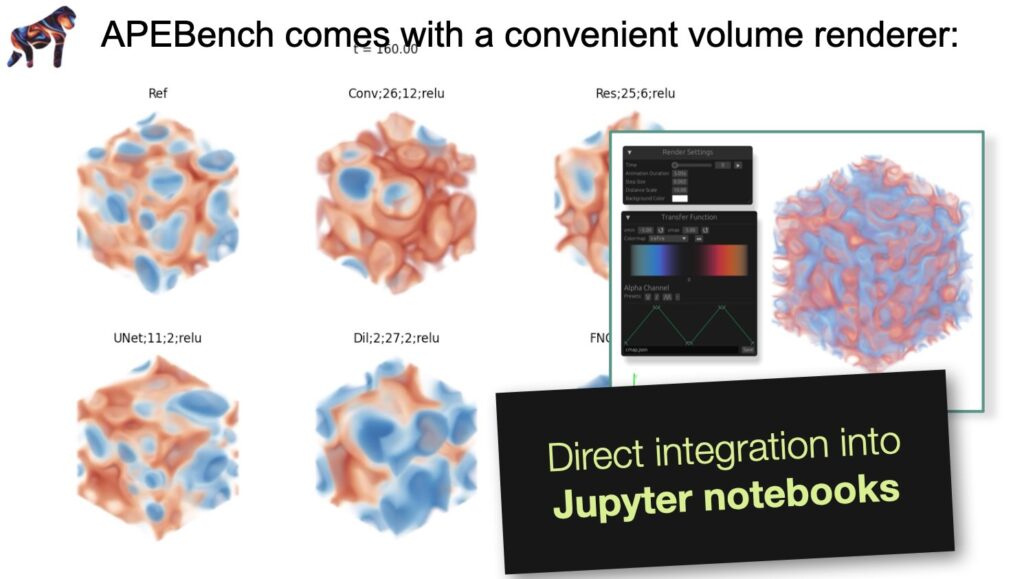
I’m excited to share our APEBench paper and the corresponding source code, to be presented at NeurIPS. Congratulations Felix and Simon 😀 👍 At its core, APEBench features a lightning-fast ⚡️ fully differentiable spectral solver with a huge range of differen PDEs.

It also comes with an integrated GPU-based volume renderer “VAPE” (https://keksboter.github.io/vape4d/), that works in your browser (and in Jupyter). If you’re patient, try it here (note – this link downloads 100MB, so it can take a moment): https://vape.niedermayr.dev/?file=https://huggingface.co/datasets/vollautomat/vape4d/resolve/main/gray_scott_3d.npy&colormap=https://huggingface.co/datasets/vollautomat/vape4d/resolve/main/colormap.json

Screenshot

Paper abstract: We introduce the Autoregressive PDE Emulator Benchmark (APEBench), a comprehensive benchmark suite to evaluate autoregressive neural emulators for solving partial differential equations. APEBench is based on JAX and provides a seamlessly integrated differentiable simulation framework employing efficient pseudo-spectral methods, enabling 46 distinct PDEs across 1D, 2D, and 3D. Facilitating systematic analysis and comparison of learned emulators, we propose a novel taxonomy for unrolled training and introduce a unique identifier for PDE dynamics that directly relates to the stability criteria of classical numerical methods. APEBench enables the evaluation of diverse neural architectures, and unlike existing benchmarks, its tight integration of the solver enables support for differentiable physics training and neural-hybrid emulators. Moreover, APEBench emphasizes rollout metrics to understand temporal generalization, providing insights into the long-term behavior of emulating PDE dynamics. In several experiments, we highlight the similarities between neural emulators and numerical simulators.

“Flow Matching for Posterior Inference with Simulator Feedback” paper online now

Our paper “Flow Matching for Posterior Inference with Simulator Feedback” is available on arXiv now: https://arxiv.org/abs/2410.22573 The key idea is to incorporate physics-constraints with guiding so that the posterior isn’t becoming biased… This gives highly accurate solutions, better than pure learning!

Code will be available at https://github.com/tum-pbs/sbi-sim

Full abstract:
Flow-based generative modeling is a powerful tool for solving inverse
problems in physical sciences that can be used for sampling and likelihood
evaluation with much lower inference times than traditional methods. We propose
to refine flows with additional control signals based on a simulator. Control
signals can include gradients and a problem-specific cost function if the
simulator is differentiable, or they can be fully learned from the simulator
output. In our proposed method, we pretrain the flow network and include
feedback from the simulator exclusively for finetuning, therefore requiring
only a small amount of additional parameters and compute. We motivate our
design choices on several benchmark problems for simulation-based inference and
evaluate flow matching with simulator feedback against classical MCMC methods
for modeling strong gravitational lens systems, a challenging inverse problem
in astronomy. We demonstrate that including feedback from the simulator
improves the accuracy by 53%, making it competitive with traditional
techniques while being up to 67x faster for inference.


Differentiability in unrolled training of neural physics simulators on transient dynamics

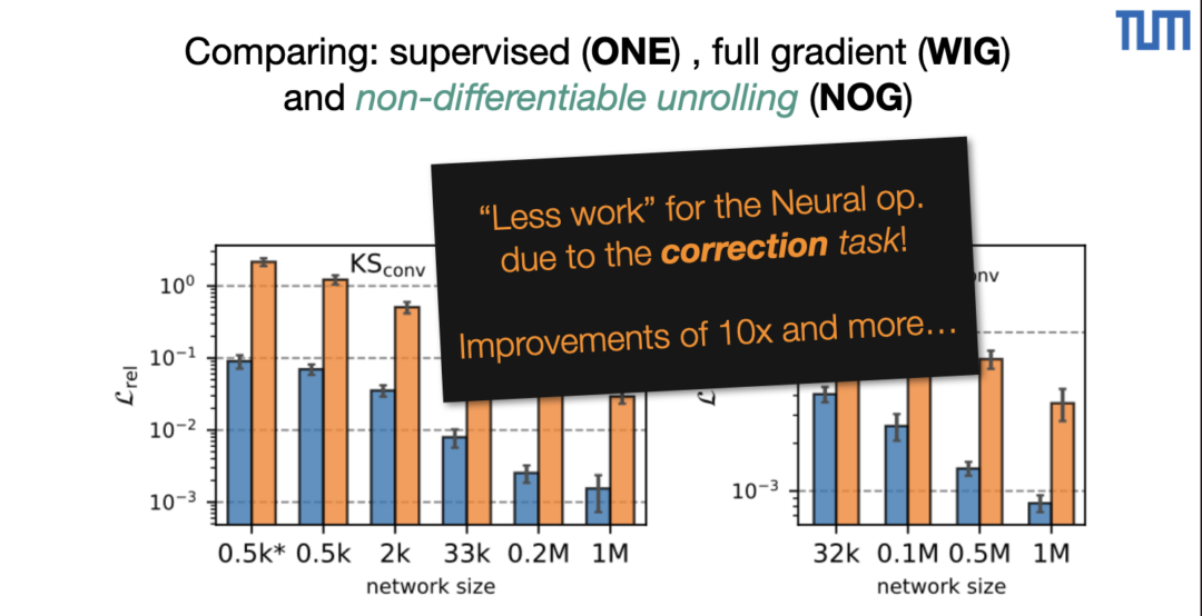
Our paper on training recurrent Neural operators with a solver-in-the-loop was now finally officially accepted at CMAME! Congratulations Bjoern 😀 👍 In parallel, we’ve been updating the paper https://arxiv.org/pdf/2402.12971 and the source code https://github.com/tum-pbs/unrolling Feel free to give it a try, and let us know how it works!

We actually have to thank the anonymous CMAME reviewers 🙏 They’ve successfully motivated us to substantially update the submission, which resulted in a big update of the paper. The theory was clarified, we included a 3D case, and with all the results being redone with relative errors the improvements are actually more substantial: moving from pure prediction to correction with unrolling yields more than 10x improvement for identical NNs.

Here’s the official CMAME link: https://authors.elsevier.com/sd/article/S0045-7825(24)00696-0

🍎 🍏 Performance comparison between NNs and numerical solvers 🍐🍍

Making a “fair” comparison between neural networks (NNs) and traditional solvers can be quite challenging and often leads to headaches 🤯. One major pitfall is comparing the NN directly with the solver used to generate the training data. In such cases, the NN will inevitably show a higher error compared to the high fidelity solver used to produce the training data. To ensure a more balanced and realistic — a “fair” — comparison, it’s essential to lower the fidelity of the solver—this gives a more accurate reflection of the NN’s performance. This is especially important when considering practical, real-world applications where we care about the accuracy produced by a chosen solver — whether it’s learned or not.

In our own work with airfoil diffusion models (https://github.com/tum-pbs/Diffusion-based-Flow-Prediction), we made finally added this more nuanced approach, adjusting the solver fidelity for a more meaningful comparison. (Shame on us that we didn’t include this in the original submission…) Even with this adjustment, we observed that the NN still delivered a 9.5x speedup on CPU compared to the classic solver (OpenFoam), and when leveraging GPU acceleration, we saw an additional order of magnitude improvement. These results highlight the significant efficiency gains achievable with neural network models, especially when accounting for the accuracy of the final output.

Please check out page 26 (Fig. 21) of our paper for details!

Flow Matching for Diffusion-based Flow Prediction of Airfoils

We have updated our diffusion-based airfoil project with flow matching https://arxiv.org/abs/2312.05320! It’s clearly better: an improved distribution with fewer iterations. Try it for yourself in our new Jupyter notebook:

https://github.com/tum-pbs/Diffusion-based-Flow-Prediction/blob/main/flow_matching.ipynb

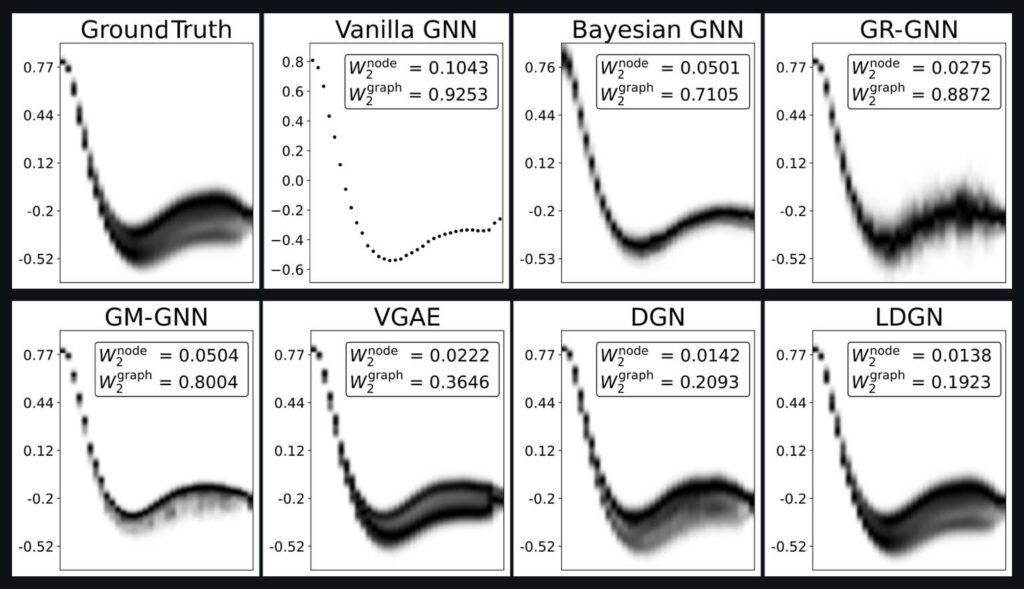
Flow Matching: We aevaluate this emerging generative modeling variant in comparison to regular diffusion models. The results demonstrate that flow matching addresses the problem of slow sampling speed typically associated with diffusion models. As such, it offers a promising new paradigm for uncertainty quantification with generative models.

For completeness, here’s the abstract of the full paper: Leveraging neural networks as surrogate models for turbulence simulation is a topic of growing interest. At the same time, embodying the inherent uncertainty of simulations in the predictions of surrogate models remains very challenging. The present study makes a first attempt to use denoising diffusion probabilistic models (DDPMs) to train an uncertainty-aware surrogate model for turbulence simulations. Due to its prevalence, the simulation of flows around airfoils with various shapes, Reynolds numbers, and angles of attack is chosen as the learning objective. Our results show that DDPMs can successfully capture the whole distribution of solutions and, as a consequence, accurately estimate the uncertainty of the simulations. The performance of DDPMs is also compared with varying baselines in the form of Bayesian neura networks and heteroscedastic models. Experiments demonstrate that DDPMs outperformthe other methods regarding a variety of accuracy metrics. Besides, it offers the advantageof providing access to the complete distributions of uncertainties rather than providing a set of parameters. As such, it can yield realistic and detailed samples from the distribution of solutions. We also evaluate an emerging generative modeling variant, flow matching, in comparison to regular diffusion models. The results demonstrate that flow matching addresses the problem of slow sampling speed typically associated with diffusion models. As such, it offers a promising new paradigm for uncertainty quantification with generative models.

Conflict-free Training for Physics Informed Neural Networks and Multi-Task Objectives

I’m excited to share our new paper: “ConFIG” https://arxiv.org/abs/2408.11104 It’s the first method for multi-task learning that really yields conflict free gradients. Whether you’re looking at PINN training or other multi-task objectives, I can highly recommend trying it out! It really beats all other methods 😃🤘 Full source code and samples are already available at: https://tum-pbs.github.io/ConFIG/

The package is now on pip: you can install via “pip install conflictfree“. Please also try the examples such as the classic PINN Burgers case: https://colab.research.google.com/github/tum-pbs/ConFIG/blob/main/docs/examples/pinn_burgers.ipynb . With a small change (providing a list of loss terms) you can directly decrease the loss from 0.031 to 0.0019. That’s 16x smaller!

Full abstract: The loss functions of many learning problems contain multiple additive terms that can disagree and yield conflicting update directions. For Physics-Informed Neural Networks (PINNs), loss terms on initial/boundary conditions and physics equations are particularly interesting as they are well-established as highly difficult tasks. To improve learning the challenging multi-objective task posed by PINNs, we propose the ConFIG method, which provides conflict-free updates by ensuring a positive dot product between the final update and each loss-specific gradient. It also maintains consistent optimization rates for all loss terms and dynamically adjusts gradient magnitudes based on conflict levels. We additionally leverage momentum to accelerate optimizations by alternating the back-propagation of different loss terms. The proposed method is evaluated across a range of challenging PINN scenarios, consistently showing superior performance and runtime compared to baseline methods. We also test the proposed method in a classic multi-task benchmark, where the ConFIG method likewise exhibits a highly promising performance. 


The Unreasonable Effectiveness of Solving Inverse Problems with Neural Networks

We just posted our paper on the “unreasonable” effectivness of NNs for optimization tasks: they outperform BFGS as a drop-in replacement when solving multiple problems. We can recommend giving it a try if you have an inverse problem where you’re currently using BFGS. We’d be very curious to hear how much improvements in terms of accuracy you get out of it!

Full paper: The Unreasonable Effectiveness of Solving Inverse Problems with Neural Networks , http://arxiv.org/abs/2408.08119

Paper abstract: Finding model parameters from data is an essential task in science and engineering, from weather and climate forecasts to plasma control. Previous works have employed neural networks to greatly accelerate finding solutions to inverse problems. Of particular interest are end-to-end models which utilize differentiable simulations in order to backpropagate feedback from the simulated process to the network weights and enable roll-out of multiple time steps. So far, it has been assumed that, while model inference is faster than classical optimization, this comes at the cost of a decrease in solution accuracy. We show that this is generally not true. In fact, neural networks trained to learn solutions to inverse problems can find better solutions than classical optimizers even on their training set. To demonstrate this, we perform both a theoretical analysis as well an extensive empirical evaluation on challenging problems involving local minima, chaos, and zero-gradient regions. Our findings suggest an alternative use for neural networks: rather than generalizing to new data for fast inference, they can also be used to find better solutions on known data.

How to Train Unconditionally Stable Autoregressive Neural Operators

Our own results on flow prediction with diffusion models, and papers from other labs, e.g., for videos and climate models, make it clear that unconditionally stable neural operators for predictions are possible. In contrast, other works for flow prediction often seem to have trouble on this front, considering fairly short horizons (and observing considerable increases of errors over time). This poses a very interesting question: which ingredients are necessary to obtain unconditional stability, meaning networks that are stable for arbitrarily long rollouts? Are inductive biases or special training methodologies necessary, or is it simply a matter of training enough different initializations? Our setup provides a very good starting point to shed light on this topic.

Based on our experiments, we start with the hypothesis that unconditional stability is “nothing special” for neural network based predictors. I.e., it does not require special treatment or tricks beyond a carefully chosen set of hyperparamters for training. As errors will accumulate over time, we can expect that network size and the total number of update steps in training are important. Our results also indicate that the architecture doesn’t really matter: we can obtain stable rollouts with pretty much “any” architecture once it’s sufficiently large.

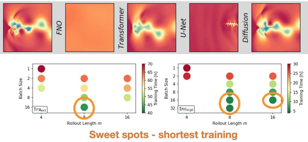
Interestingly, we find that the batch size and the length of the unrolling horizon play a crucial role. However, they are conflicting: small batches are preferable, but in the worst case under-utilize the hardware and require long training runs. Unrolling on the other hand significantly stabilizes the rollout, but leads to increased resource usage due to the longer computational graph for each NN update. Thus, our experiements show that a “sweet spot” along the Pareto-front of batch size vs unrolling horizon can be obtained by aiming for as-long-as-possible rollouts at training time in combination with a batch size that sufficiently utilizes the available GPU memory.

Learning Task: To analyze the temporal stability of autoregressive models on long rollouts, two flow prediction tasks from our ACDM benchmark are considered: an easier incompressible cylinder flow (Inc), and a complex transonic wake flow (Tra) at Reynolds number 10 000. For Inc, the models are trained on flows with Reynolds number 200 – 900 and required to extrapolate to Reynolds numbers of 960, 980, and 1000 during inference (Inchigh). For Tra, the training data consists of flows with Mach numbers between 0.53 and 0.9, and models are tested on the Mach numbers 0.50, 0.51, and 0.52 (Traext). For each sequences in both data sets, three training runs of each architecture are unrolled over 200 000 steps. This unrolling length is of course no proof that these networks yield infinitely long stable rollouts, but from our experience they feature an extremely small probability for blowups.

Architectures: As a first comparison, we train three model architectures with an identical backbone U-Net (as a representative of convolutional and discrete neural operators), that use different stabilization techniques. This comparison shows that it is possible to successfully achieve the task “unconditional stability” in different ways:

  1. Unrolled training (U-Netut) where gradients are backpropagated through multiple time steps during training.
  2. Models trained on a single prediction step with added training noise (U-Nettn). This technique is known to improve stability by reducing data shift, as the added noise emulates errors that accumulate during inference.
  3. Autoregressive conditional diffusion models (ACDM). A DDPM-like model is conditioned on the previous time step and iteratively refines noise to create a prediction for the next step. The resulting predictor is then autoregressively unrolled for a full simulation rollout.

Figure 1: Vorticity predictions for an incompressible flow with a Reynolds number of 1000 (top) and for a transonic flow with Mach number 0.52 (bottom) over 200 000 time steps.

Figure 1 above illustrates the resulting predictions. All methods and training runs remain unconditionally stable over the entire rollout on Inchigh. Since this flow is unsteady but fully periodic, the results of all models are simple, periodic trajectories that prevent error accumulation. For the sequences from Traext, one from the three trained U-Nettn models has stability issues within the first few thousand steps and deteriorates to a simple, mean flow prediction without vortices. U-Netut and ACDM on the other hand are fully stable across sequences and training runs for this case, indicating a fundamentally higher resistance to rollout errors which normally cause instabilities. The autoregressive diffusion models turn out to be unconditionally stable across the board, so we’ll drop them in the following evaluations and focus on models where stability is more difficult to achieve: the U-Nets as representatives of convolutional, discrete neural operators.

Stability Criteria: Focusing on the U-Net networks with unrolled training, we will next focus on training multiple models (3 each time), and measure the percentage of stable runs they achieve. This provides more thorough statistics compared to the single, qualitative examples above. We’ll investigate the first key criterium rollout length, to show how it influences fully stable rollouts over extremely long horizons. Figure 2 lists the percentage of stable runs for a range of ablation models on the Traext data set with rollouts over 200 000 time steps. Results on the indiviual Mach numbers, as well as an average are shown.

Figure 2: Percentage of stable runs on the Traext data set for different ablations of unrolled training.

The most important criterion for stability is the number of unrolling steps m: while models with m <= 4 do not achieve stable rollouts, using m >= 8 is sufficient for stability across different Mach numbers. Three factors that did not substantially impact rollout stability in our experiments are the prediction strategy, the amount of training data, and the backbone architecture. First, using residual predictions, i.e., predicting the difference to the previous time step instead of the full time steps itself, does not impact stability. Second, the stability is not affected when reducing the amount of available training data by a factor of 8 from 1000 time steps per Mach number to 125 steps (while training with 8× more epochs to ensure a fair comparison). This training data reduction still retains the full physical behavior, i.e., complete vortex shedding periods. Third, it possible to train other backbone architectures with unrolling to achieve fully stable rollouts as well, such as dilated ResNets. For ResNets without dilations only one trained model is stable, most likely due to the reduced receptive field. However, we expect achieving full stability is also possible with longer training rollout horizons.

Batch Size vs Rollout: Furthermore, we observed that the batch size can impact the stability of autoregressive models. This is similar to the image domain where smaller batches are know to improve generalization, which is the motivation for using mini-batching instead of gradients over the full data set. The impact of the batch size on the stability and model training time is shown in Figure 3, for both investigated data sets. Models that only come close to the ideal rollout lenght at a large batch size, can be stabilized with smaller batches. However, this effect does not completely remove the need for unrolled training, as models without unrolling were unstable across all tested batch sizes. Note that models with smaller batches were trained for an equal number of epochs, as an identical number of network updates did not improve stability. For the Inc case, the U-Net width was reduced by a factor of 8 across layers to artifically increase the difficulty of this task, as otherwise all parameter configurations would already be stable.

Figure 3: Percentage of stable runs and training time for different combinations of rollout length and batch size. Shown are results from the Traext data set (top) and the Inchigh data set (bottom). Grey configurations are omitted due to memory limitations (mem) or due to high computational demands (-).

Increasing the batch size is more expensive in terms of training time on both data sets, due to less memory efficient computations. Using longer rollouts during training does not necessarily induce longer training times, as we compensate for longer rollouts with a smaller number of updates per epoch. E.g., we use either 250 batches with a rollout of 4, or 125 batches with a rollout of 8. Thus the number of simulation states that each model sees over the course of training remains constant. However, we did in practice observe additional computational costs for training the larger U-Net model on Traext. This leads to the question which combination of rollout length and batch size is most efficient.

Figure 4: Training time for different combinations of rollout length and batch size to on the Traext data set (left) and the Inchigh data set (right). Only configurations that to lead to highly stable models (stable run percentage >= 89%) are shown.

Figure 4 shows the central tradeoff between rollout length and batch size (only stable versions included here). To achieve unconditionally stable neural operators, it is consistently beneficial to choose configurations where large rollout lengths are paired with a batch size that is big enough the sufficiently utilize the available GPU memory. This means, improved stability is achieved more efficiently with longer training rollouts rather than smaller batches, as indicated by the green dots with the lowest training times.

Summary: With a suitable training setup, unconditionally stable predictions with extremely long rollout are possible, even for complex flows. According to our experiments, the most important factors that impact stability are:

  • Long rollouts at training time
  • Small batch sizes
  • Comparing these two factors: longer rollouts result in faster training times than smaller batch sizes
  • At the same time, sufficiently large models are necessary, depending on the complexity of the learning task.

Factors that did not substantially impact long-term stability are:

  • Prediction paradigm during training, i.e., residual and direct prediction are viable
  • Additional training data without new physical behavior
  • Different backbone architectures, even though the ideal number of unrolling steps might vary for each architecture

Further information on these experiments can be found in our paper https://arxiv.org/abs/2309.01745 and visualizations of trajectories with shorter rollout on our project page https://ge.in.tum.de/publications/2023-acdm-kohl/.

ICML 2024 Workshops

ICML ’24 is over, but for all those who didn’t have a chance to enjoy and study our workshop submission in more detail – this is your chance. Below you can find all five workshop submissions in their full glory. If any questions come up, feel free to contact us, of course!

Our works covered a large ground in scientific machine learning, i.e., combinations of numerical simulations and deep learning techniques. In summary, we covered:

You can follow each of the links to view the full poster. Enjoy!

The Unreasonable Ineffectivness of NN-Accuracy Scaling

TL;DR: There’s a surprising aspect of our recent paper https://arxiv.org/abs/2402.12971 that’s easy to overlook: we noticed that NN test error scales sub-optimally with -1/3 over parameter count. This is for correction, while prediction tasks are slightly worse with -1/4. Our results indicate that this is stable across physical systems and network architectures!

To provide more background: many experiments from our paper “How Temporal Unrolling Supports Neural Physics Simulators” https://arxiv.org/abs/2402.12971 show clear, continuous improvements in accuracy for increasing network sizes.

An obvious conclusion is that larger networks achieve better results. However, in the context of scientific computing, simply increasing the network size further and further is not an attractive option. As neural approaches compete with established numerical methods, applying pure neural or hybrid architectures always entails accuracy, efficiency, and scaling considerations. The scaling of networks towards real-world engineering problems on physical systems has been an open question, and overly large networks will be more resource hungry than established solvers in the worst case.

To shed light here, we computed a convergence rate between the test loss and the number of network parameters. We used an average test loss for each individual combination of network size and training setup. The average is computed over the full set of random seeds used in our study, i.e., 8 to 20 individual training runs per size and variant depending on the physical system (more than 800 models for the 3 graphs above). For the correction setups (NN+coarse solver), we estimate the convergence rate of the correction networks with respect to the parameter count n to be n^-1/3, as shown above. This means a network with twice the size only gives an error reduction of ca. 20% … that’s not a lot.

Interestingly, the measured convergence rates are agnostic to the physical system and the studied network architectures. For prediction setups (pure NN, no solver), the convergence rate of the networks with respect to the parameter count n is even slightly worse with n^-1/3 , as shown below.

Interestingly, even for larger “foundation-model” networks there seems to be a similar scaling for the accuracy over parameters: here’s a comparison with the Poseidon paper (very interesting: https://arxiv.org/abs/2405.19101) which uses a transformer architecture , side-by-side with our experiments with a simpler ConvNet (same as above). We saw n^-1/4 , there it seems closer to n^-1/6:

Conclusions: This convergence rate is poor compared to classic numerical solvers, and indicates that neural networks are best applied for their intrinsic benefits. They possess appealing characteristics like data-driven fitting, reduced modeling biases, and flexible applications. In contrast, scaling to larger problems is more efficiently achieved by numerical approaches. In applications, it is thus advisable to combine both methods to render the benefits of both components. It also motivates the correction hybrids, where a NN supports a numerical solver. These achieve much higher accuracies, the solver can take care of the large scale generalization, and the NN can be correspondingly smaller.

For details, please check out the full paper at: https://arxiv.org/abs/2402.12971

Talk about Diffusion Models for Probabilistic Neural Solvers

Here’s also a talk summarizing our recent work on diffusion models for probabilistic Neural solvers: https://youtu.be/xaWxERImy0g

It covers the whole range: from steady state cases, over time-dependent surrogate models, all the way to integrating differentiable simulations into learning score functions. And here are the three corresponding papers:

How to accurately evaluate whether a diffusion model learned the right distribution?

This is a tough task, as many existing data sets for generative models come without quantifiable ground truth data. In contrast the 1D airfoil case of our recent AIAA paper is highly non-trivial but comes with plenty of GT data. Thus, it’s easy to check whether a neural network such as a diffusion model learned the correct distribution of the solutions (by computing the “coverage” in terms of distance to the GT solutions), and to check how much training data is needed to actually converge.

Here’s a Jupyter notebook that explains how to use it: https://colab.research.google.com/github/tum-pbs/Diffusion-based-Flow-Prediction/blob/main/sample.ipynb

The image below shows the content of the data set: the input is a single parameter, the Reynolds number, and with increasing Re the complexity of the solutions rises, and starts to vary more and more. The mean on the left hand side stays largely the same, while the increasing and changing standard deviation of the solutions (show on the right) highlights the enlarged complexity of the solutions. Intuitively, the low Re cases have flows that mostly stick to the mean behavior, while the more turbulent ones have a larger number of different structures from more and more complex vortex shedding. As a consequence, a probabilistic neural network trained on this case will need to figure out how the solutions change along Re. Also, it will need to figure out how to generate the different modes of the solutions that arise for larger Re cases.

For details and comparisons with other approaches, please check out section (B) of the paper. The data of the 1D case itself is checked in at https://github.com/tum-pbs/Diffusion-based-Flow-Prediction/tree/main/datasets/1_parameter.

Neural solvers for wake flows at Physical Review E

We’re glad to report that Physical Review E has just accepted our paper on neural solvers for wake flows and boundary layers. You can find the full preprint here https://arxiv.org/abs/2308.04296 , and source code is available at https://github.com/tum-pbs/DiffPhys-CylinderWakeFlow/.

Full paper abstract: This work delineates a hybrid predictive framework configured as a coarse-grained surrogate for reconstructing unsteady fluid flows around multiple cylinders of diverse configurations. The presence of cylinders of arbitrary nature causes abrupt changes in the local flow profile while globally exhibiting a wide spectrum of dynamical wakes fluctuating in either a periodic or chaotic manner. Consequently, the focal point of the present study is to establish predictive frameworks that accurately reconstruct the overall fluid velocity flowfield such that the local boundary layer profile, as well as the wake dynamics, are both preserved for long time horizons. The hybrid framework is realized using a base differentiable flow solver combined with a neural network, yielding a differentiable physics-assisted neural network (DPNN). The framework is trained using bodies with arbitrary shapes, and then it is tested and further assessed on out-of-distribution samples. Our results indicate that the neural network acts as a forcing function to correct the local boundary layer profile while also remarkably improving the dissipative nature of the flowfields. It is found that the DPNN framework clearly outperforms the supervised learning approach while respecting the reduced feature space dynamics. The model predictions for arbitrary bodies indicate that the Strouhal number distribution with respect to spacing ratio exhibits similar patterns with existing literature. In addition, our model predictions also enable us to discover similar wake categories for flow past arbitrary bodies. For the chaotic wakes, the present approach predicts the chaotic switch in gap flows up to the mid-time range.

Deep learning-based predictive modeling of transonic flow over aerofoils

Our work on transonic flows over aerofoils is finally online: https://arxiv.org/abs/2403.17131

Apart from being accurate & stable. We also realized the trained models allow for efficiently performing a “classic” global instability analysis.

It was great to see the networks “really” learn the fundamental physics: When applied to a previously unseen mean flow, the eigenvalue spectrum of the trained network reliably captures the key modes that we’d expect from a transient case.

The unstable modes near 10^-1 along y (with positive real part) indicate the onset of buffet, i.e. growing large scale instabilities in the flow. The smaller modes around 2*10^0 are typical vortex shedding frequencies from the Kelvin-Helmholtz instability.

Full paper abstract: Effectively predicting transonic unsteady flow over an aerofoil poses inherent challenges. In this study, we harness the power of deep neural network (DNN) models using the attention U-Net architecture. Through efficient training of these models, we achieve the capability to capture the complexities of transonic and unsteady flow dynamics at high resolution, even when faced with previously unseen conditions. We demonstrate that by leveraging the differentiability inherent in neural network representations, our approach provides a framework for assessing fundamental physical properties via global instability analysis. This integration bridges deep neural network models and traditional modal analysis, offering valuable insights into transonic flow dynamics and enhancing the interpretability of neural network models in flowfield diagnostics.

Learning Symmetric Basis Convolutions at ICLR’24

Our ICLR’24 paper on learning Fourier-based convolutions (SFBC) for particle and unstructured data is online now on arXiv: https://arxiv.org/abs/2403.16680

A first version of the SFBC source code is also up at https://github.com/tum-pbs/SFBC , the approach is especially interesting as an inductive bias for accurate neural networks, e.g. to replace graph-nets.

The graph above shows a quantitative evaluation of different network architectures for a fixed layout with four message-passing steps and 32 features per layer. It’s noticeable that the Fourier-convolutions (SFBC) clearly outperform the graph-net based methods (MLPCConv, GNS and MP-PDE on the right). We noticed this is many settings: for a given parameter budget, the inductive bias of the convolutions helps the network to correlate spatial features, and to give more accurate results.

Visual Flow Capture with Raspberry Pi

For TUM students: we also have a new thesis topic on visual flow capture with RPIs. This is motivated by a previous project: ScalarFlow. There we created a first large-scale data set of reconstructions of real-world smoke plumes. It used an accurate physics-based reconstruction from a small number of video streams. Central components of our framework were a novel estimation of unseen inflow regions and an efficient optimization scheme constrained by a simulation to capture real-world fluids. The published data set contains volumetric reconstructions of velocity and density as well as the corresponding input image sequences.

More info can be found here: https://ge.in.tum.de/download/thesis-MA-rpi.pdf

If you have experience with hardware setups and cameras, please contact us via email at i15ge@cs.tum.edu . We have thesis and or HiWi positions available in this area!

How Temporal Unrolling Supports Neural Physics Simulators on arXiv

It’s worth pointing out that our paper on “How Temporal Unrolling Supports Neural Physics Simulators” is online now: https://arxiv.org/abs/2402.12971

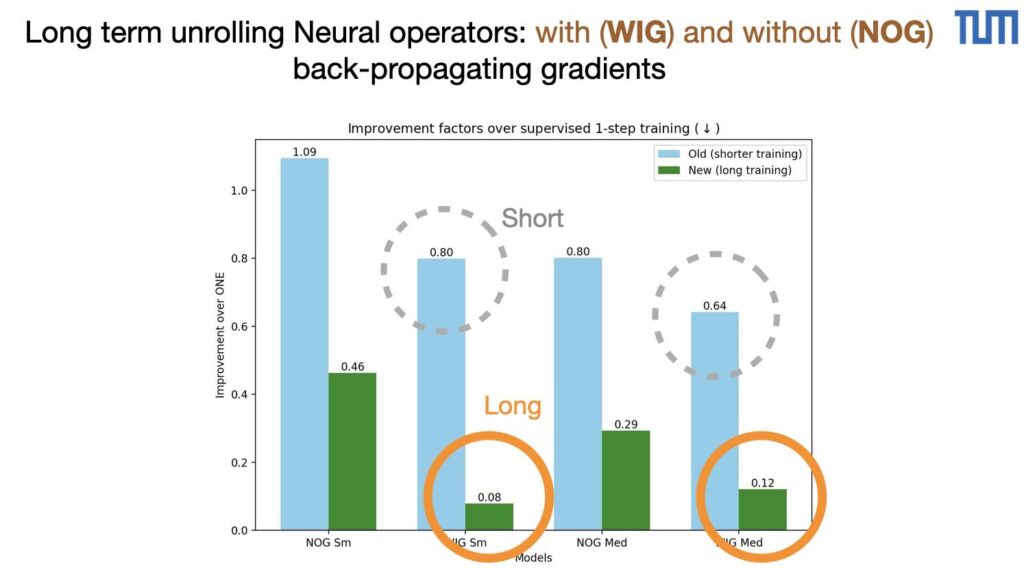
One of the key findings is: don’t throw away your simulator (yet) even if it doesn’t have gradients. You can get substantial accuracy boosts (around 5x) by coupling an NN with the simulator, instead of letting the NN do all the work… Here are results for a KS and a turbulence case:

Paper Abstract: Unrolling training trajectories over time strongly influences the inference accuracy of neural network-augmented physics simulators. We analyze these effects by studying three variants of training neural networks on discrete ground truth trajectories. In addition to commonly used one-step setups and fully differentiable unrolling, we include a third, less widely used variant: unrolling without temporal gradients. Comparing networks trained with these three modalities makes it possible to disentangle the two dominant effects of unrolling, training distribution shift and long-term gradients. We present a detailed study across physical systems, network sizes, network architectures, training setups, and test scenarios. It provides an empirical basis for our main findings: A non-differentiable but unrolled training setup supported by a numerical solver can yield 4.5-fold improvements over a fully differentiable prediction setup that does not utilize this solver. We also quantify a difference in the accuracy of models trained in a fully differentiable setup compared to their non-differentiable counterparts. While differentiable setups perform best, the accuracy of unrolling without temporal gradients comes comparatively close. Furthermore, we empirically show that these behaviors are invariant to changes in the underlying physical system, the network architecture and size, and the numerical scheme. These results motivate integrating non-differentiable numerical simulators into training setups even if full differentiability is unavailable. We also observe that the convergence rate of common neural architectures is low compared to numerical algorithms. This encourages the use of hybrid approaches combining neural and numerical algorithms to utilize the benefits of both.

Differentiable simulation library Phi-ML at JOSS

The differentiable simulation library ΦML (Phi-ML), which is e.g. the basis for projects like PhiFlow, has been accepted in JOSS now! Congratulations Philipp 😀 👍 The full version is available here: https://joss.theoj.org/papers/10.21105/joss.06171

Short summary: ΦML is a math and neural network library designed for science applications. It enables you to quickly evaluate many network architectures on your data sets, perform linear and non-linear optimization, and write differentiable simulations. ΦML is compatible with JaxPyTorchTensorFlow and NumPy and your code can be executed on all of these backends.