When explaining differentiable physics training, the following question regularly comes up: “So, how much does training with this differentiable physics simulator really improve things? E.g., compared to unrolling a supervised setup?” In short, a lot! Here’s the answer for a nice turbulent mixing layer case (all from Björn’s paper, available as a preprint at https://arxiv.org/abs/2202.06988).
First, we can qualitatively show the differences. Here’s the DNS reference version compared to a full differentiable physics training with 10 steps, and the “supervised unrollment” version. The latter has the back propagation through the solver disabled, but is identical otherwise :
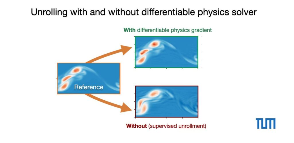
It’s quite obvious that the long-term feedback through the solver is missing for the supervised version. It produces noticeable artifacts and oscillations. Note that both versions still use a powerful set of carefully selected turbulence losses, as described in the paper. Otherwise the difference would be even larger.
We can also quantify these differences in terms of the resolved Reynolds stresses:
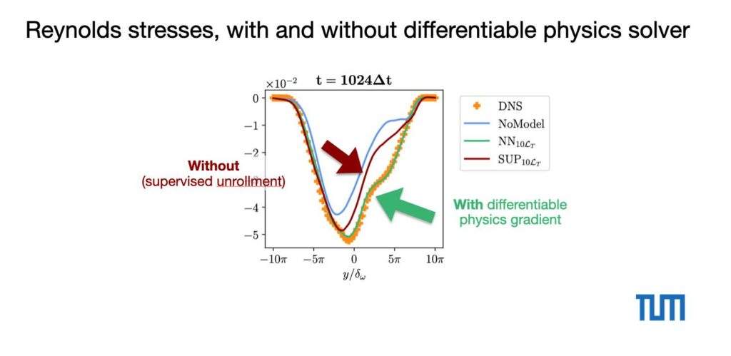
The ground truth targets are shown as orange dots here. There’s a clear gap that the differentiable physics training can close towards the reference.
And here for the resolved turbulent kinetic energy. On the positive side of the graph, the DP version aligns better with the ground truth:
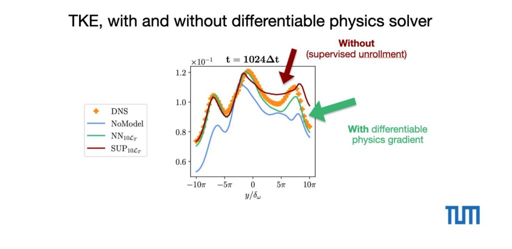
All of these results are from a very late time step: after evaluating 1024 time steps with the hybrid solver, i.e., alternating evaluations of the PISO solver and the trained neural network turbulence model. With a carefully chosen learning setup, even the supervised model stays stable for this time span, but the model nonetheless does significantly better when it receives the long-term feedback in the form of gradients from the differentiable flow solver.
To summarize, the unrollment of time steps with differentiable physics training gives significant gains for the accuracy of neural network powered solvers. Especially when such a NN-based turbulence model is to be trained once, and then deployed and evaluated many times in an application, the one time cost to train the model together with the solver will amortize very quickly.