So, let’s start with an example that’s as simple as possible: a very simple mantaflow scene that generates some flow data, and a simple tensorflow setup that trains a simple neural network with this data. Such a setup can be found as part of mantaflow under “mantaflow/tensorflow/example0_simple”. This example demonstrates how to generate flow data sets with mantaflow, and then trains a simplistic auto encoder using a smoke density data set. An auto encoder (AE) is a particularly convenient way to start, as AEs simply learn a reduced latent space representation of a data set, from which the original signal should be reconstructed as accurately as possible. If you’re interested in the details of AEs, you can, e.g., find more info on Wikipedia (https://en.wikipedia.org/wiki/Autoencoder) and in the references on that page.
Note that each of the mantaflow examples comes with a short README.txt file that briefly summarizes the steps to run the example. In the following, we’ll go into a bit more detail though. It’s also worth pointing out that the python files with a “manta_” prefix are supposed to be run with mantaflow, while the “tf_” files can simply be executed in python. As mantaflow was initially intended as a stand-alone simulator it’s currently not available as a python library. Instead, the mantaflow executable provides the simulator functionality upon loading, hence the difference between the two types of python files.
Getting Data to Train with…
The simple example only contains two python files: “manta_genSimSimple.py” to generate the flow data, and “tf_simple.py” which contains the network setup and training code. Naturally, the data generation comes first. This setup is a simple smoke simulation at its core (the advectSemiLagrange, addBuoyancy, and solvePressure calls in the main loop). We won’t discuss the details of the smoke simulation here, if you’re interested in that part, please check out the mantaflow scene tutorial at http://mantaflow.com/scenes.html. In addition to the smoke sim, the manta_genSimSimple scene initializes several randomized density sources and two velocity sources with randomized directions. The density sources are created in the “for nI in range(noiseN)” loop, and the velocity sources are initialized right below.
All mantaflow examples store their data in a “base directory”, the basePath variable, which by default is set to “../data”. All the examples also assume that they’re run from the directory in which the python scripts are located. Thus, make sure to change into the right directory, e.g., with “cd mantaflow/tensorflow/example0_simple”, before starting the scene with “…/manta ./manta_genSimSimple.py”. Note that this scene (and those from the other examples) take an optional command line parameter “seed“, which can be used to deterministically create randomized data sets. By default, a random initial seed is used in numpy, so when calling without any additional parameters, the scene will generate a random data set, and save the data in “../data/simSimple_XXXX”, where XXXX is replaced by the first free available index (starting with an index of 1000). After the run, you’ll find a sequence of “density_” and “vel_” .uni files in this directory. The .uni files are mantaflow’s own custom format for saving grid and particle data. It’s a relatively simple gzipped binary format, with a bit of header information, and represents the easiest way to read and write data in mantaflow.
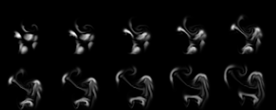
Fig. 1: A sequence of example density configurations produced by the data generation script.
For deep learning tasks, you’ll generally need as much data as possible. For this mantaflow example, you can simply run the generation script a few times, e.g., ten times, to generate a fair number of simulation data sets. As the task is training an auto encoder, having more variance in the data will actually make the task harder, so it’s not advisable to generate much more than that (unless you make the network larger). Afterwards, you should find the ca. ten “simSimple_” directories in your “../data/” directory. If those exist, you’re set to start training a first neural network with the data.
Making the Network Learn
For this setup, training the NN is actually very simple: just run the “tf_simple.py” script in python. Note that a common initial pitfall is having multiple python versions installed (e.g., 2.x and 3.y), and calling the wrong one. The scripts should work with 2 and 3, but we’d highly recommend to only use a single one in practice. The tensorflow script itself is worth a closer look. The first important bit is loading the mantaflow data, and preparing it for training.
Loading the simulation data is the first important step in this file. In this simple example, this is done in a very straight forward manner. The script simply looks for directories with indices in the range of 1000 to 2000, and then loads 100 .uni density files from each of them using the “readUni” function of the uniio module (in “../tools”). This function returns a header and the grid data as a numpy array. In the code snippet below you can find this loop, together with code to retrieve x and y dimension from the uni file header:
for sim in range(1000,2000):
     if os.path.exists( "%s/simSimple_%04d" % (basePath, sim) ):
     for i in range(0,100):
          filename = "%s/simSimple_%04d/density_%04d.uni"
          uniPath = filename % (basePath, sim, i)
          header, content = uniio.readUni(uniPath)
          h = header['dimX']
          w = header['dimY']
Width and height come in handy in order to reshape the array. By default, the readUni function always returns an array of the shape ZYXC, where ZYX are the spatial dimensions, and C the channels per cell. For a scalar grid (originally of type RealGrid in mantaflow), we’ll have a single value, i.e., C=1. Thus in this case readUni will return an array of shape [1,64,64,1]. The next lines make sure the arrays have the right shape, and it simplifies writing images.
This is worth explaining in more detail. Theoretically, we could work with the ZYXC arrays after loading them, but for a pure 2D example, it unnecessarily complicates things if we have to drag around the Z axis. Thus, we can simply reshape the array to discard the Z axis, which works fine as long as we make sure we only have a single 2D slice in the array.
In addition, mantaflow assumes the origin (0,0) is in the bottom left corner when showing grids in the UI. On the other hand, for image output its pretty common to have the (0,0) point in the top right corner. So, in order to make sure we can simply write out any array as an image, and to get a look similar to mantaflow, we can use some python slicing magic to reverse the array content along the Y axis. While the [::] slice notation in the code below might look strange at first, it’s a powerful tool that you’ll encounter in many numpy and tensorflow examples, so it’s worth getting used to it. E.g., check out https://docs.scipy.org/doc/numpy/reference/arrays.indexing.html for further details. In short, we can write “start:stop:step” to specify a range. If some of these are left out, numpy simply inserts the defaults. Thus “::-1” goes across the whole length of an axis, with a reverse step of -1. Finally, the array is appended to the densities variable, which is simply a list of array objects that is used later on for training the network.
arr = arr[:, ::-1, :, :]
arr = np.reshape(arr, [w, h, 1])
densities.append( arr )
Next, we’ll slice up the data into at least one full simulation as validation data set (or 10% of all data if we have enough), while the rest will be used for training.
loadNum = len(densities)valiSize = max(100, int(loadNum * 0.1))
valiData = densities[loadNum-valiSize:loadNum,:]
densities = densities[0:loadNum-valiSize,:]
Now we can go ahead and set up the network. As outlined above, we’re using a simple auto encoder. In the following x will denote the inputs, while y will be the “ground truth” value, i.e., the correct output which we’d like the network to compute as accurately as possible. Thus, we’re trying to represent the function f for f(x)=y. We’re first defining placeholders with the same size as our density grids, adding another dimension for the batch size. For details about setting up neural networks with tensorflow, check out the official resources, e.g., the MNIST example at https://www.tensorflow.org/get_started/mnist/beginners. In short, we’re allocating a single fully connected layer of size 50, before re-creating the full output of size [64,64,1] as y_pred. You can find an summary of the network architecture in the following picture.
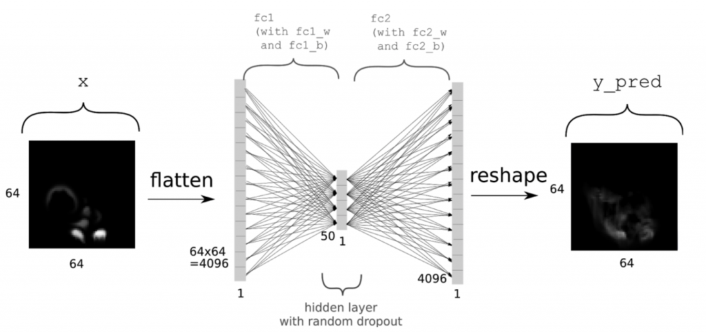
(Thanks to Daniel Hook for the image)
Note that we’re directly including a fair amount of dropout with a rate of 0.5 for the fully connected layer fc1. As activation function, we’re using tanh here, and as the final output in y_pred is the final output of the network, we’re not applying an activation function to it. All that’s done to y_pred is reshaping it into grid form.
x = tf.placeholder(tf.float32, shape=[None, 64,64, 1])
y = tf.placeholder(tf.float32, shape=[None, 64,64, 1])
inSize = 64 * 64 * 1
xIn    = tf.reshape(x, shape=[-1, inSize ])

fc_1w  = tf.Variable(tf.random_normal([inSize, 50], stddev=0.01))
fc_1b  = tf.Variable(tf.random_normal([50], stddev=0.01))

fc1 = tf.add(tf.matmul(xIn, fc_1w), fc_1b)
fc1 = tf.nn.tanh(fc1)fc1 = tf.nn.dropout(fc1, 0.5)

fc_2w = tf.Variable(tf.random_normal([50, inSize], stddev=0.01))
fc_2b = tf.Variable(tf.random_normal([inSize], stddev=0.01))

y_pred = tf.add(tf.matmul(fc1, fc_2w), fc_2b)
y_pred = tf.reshape( y_pred, shape=[-1, 64, 64, 1])
Loss function and optimizer are pretty straight-forward: a simple L2 loss, and the popular ADAM optimizer with a small enough step size:
cost = tf.nn.l2_loss(y - y_pred)
opt  = tf.train.AdamOptimizer(0.0001).minimize(cost)
Now we have all parts in place to train the network. We can set up a tensorflow session, and start out training epoch loop. Note that while an “epoch” usually denotes a full pass over the training data, we’re using it to denote training iterations here. Despite trying to keep things simple, we shuffle the entries of our batches to avoid bias in the computed gradients. This is done in a very simple way, by generating random indices into our training array, and appending the selected arrays to the current batch. We’re using a fixed batch size of 10 in this script. The batch is then fed into x using tensorflow’s “feed_dict” functionality.
sess = tf.InteractiveSession()
sess.run(tf.global_variables_initializer())
for epoch in range(trainingEpochs):
    c = (epoch * batchSize) % densities.shape[0]
    batch = []
    for currNo in range(0, batchSize):
        r = random.randint(0, loadNum-1)
        batch.append( densities[r] )
    _ , currentCost = sess.run([opt, cost], feed_dict={x: batch, y: batch})
The most interesting call here is sess.run, which executes a full forward and backward pass through the network, in order to update the weights. Note that all variables passed in the first list “[opt,cost]” are evaluated, and their respective values returned by sess.run. In this example, we’re ignoring the return value of the optimizer, by using the underscore placeholder in “_,currentCost”. We’re only storing the cost such that we can keep track of training progress if necessary. While repeatedly calling sess.run with randomized batches would be enough to train the network, it’s typically crucial to evaluate how well the network generalizes to new data. In this example, we run the trained network on our validation data every 10 update steps
[valiCost,vout] = sess.run([cost, y_pred], feed_dict={x: valiData, y: valiData})
For this sess.run call we don’t need to evaluate the optimizer, but we simply check the cost computed with the L2 distance between ground truth y and prediction y_pred. In addition, we’re storing the generated arrays in the variable vout. This is not strictly necessary for training. Instead, it only simplifies writing the results to disk at the end of training. When you run this example, you should see an output such as this one on your screen:
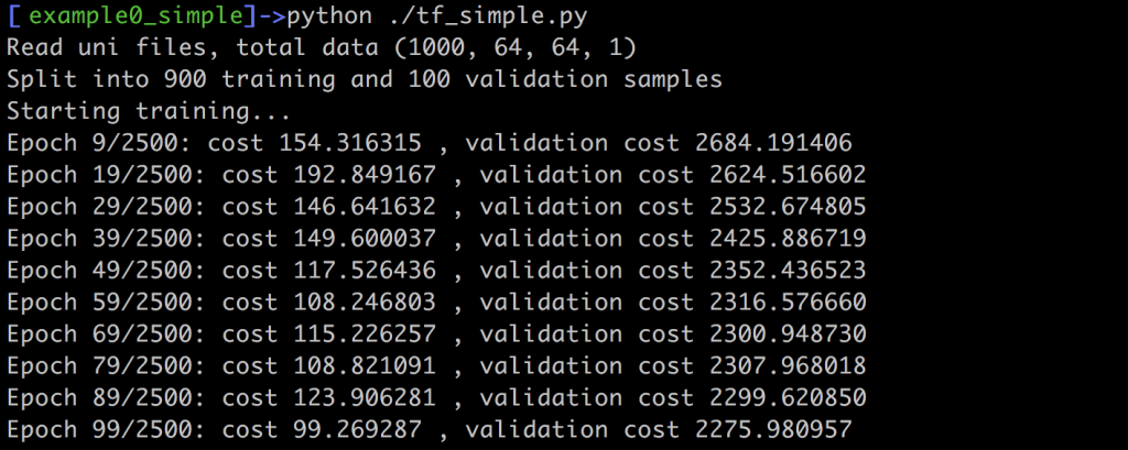
The command line output should give you a rough feedback about how the network does on the training and validation data. In this example, the L2 norm is not normalized w.r.t. the number of inputs, thus the larger number of validation samples lead to much larger values. Still, whatever the absolute values are in your case, both costs should slowly decrease over the course of the training iterations. Once we’ve reached the last iteration, this script outputs the whole validation data set as png images, using scipy’s toimage function:
for i in range(len(valiData)):
    scipy.misc.toimage( np.reshape(valiData[i], [64, 64]) , cmin=0.0, cmax=1.0).save("in_%d.png" % i)
    scipy.misc.toimage( np.reshape(vout[i]    , [64, 64]) , cmin=0.0, cmax=1.0).save("out_%d.png" % i)
Thus, after the script is done, you should find ca. 100 in_XXX.png images showing the inputs, and 100 out_XXX.png images showing the corresponding reconstruction of the network. Below you can find an example of what to expect from the default settings. You’ll notice that the reconstructions don’t match the inputs very closely, but you should be able to roughly see the input shape, nonetheless. Also, keep in mind, that the latent space (the size of the hidden layer) of this network is only 50! That less than 2% of the input size (which was 64*64), and for the chaotic density inputs from our flow simulations, the network does a pretty good job of reconstructing the inputs from only those 50 scalars.
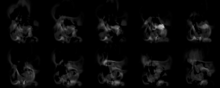 Fig. 2: Outputs generated by the network (note – the brightness was increased a bit to make things easier to see).
Wrap-up
This concludes this “as-simple-as-possible” example. There are many ways in which you could improve and extend this setup. E.g., try different amounts of input data, different hidden layer sizes, different optimizers/activation functions, or add multiple hidden layers. Somewhat more advanced: you could add convolutional layers (more on that in the next chapters), or turn the auto encoder into a variational one to improve the shape of the latent space and typically also the reconstructions.